ARIMA
date posted: 2020-10-11
Time series
Data points that are observed at specified times usually at equal intervals are referred to as time series data. Time series is very important in real life since most data are measured in time consequtive manner. Ex: Stock prices being recorded every second.
Time series analysis are used to predict the future. For example using past 12 months sales data to predict next n month sales therefore we could act accordingly.
Four components that explains time series data:
- Trend : Upward, downward, or stationary. If your company sales increase every year it is showing an upward trend.
- Seaonality: Repeating pattern in certain period. Ex: difference between summer and winter. Also includes special holidays
- Irregularity: External factors that affect time series data such as Covid, natural disasters.
- Cyclic: repeating up and down time series data.
ARIMA
Auto Regressive Integrated Moving Average
a.k.a Box-Jenkins method.
- It is class of models that forecase using own past values: lag values and lagged forecast errors.
- AR model uses lag values to forecast
- MA model uses lagged forecast errors to forecast
- Two models Integrated becomes ARIMA
- Consists of three parameters: p, q, d
It is a naive model since it assumes time series data are:
- "non-seasonal" meaning different seasons do not affect its values. When there exists seasonality we use SARIMA short for Seasonal ARIMA model
- Has no Irregularity
Parameters
p - order of AR termNumber of lags of Y to be used as predictors. In other words, If you are trying to predict June's sale how many previous(lag) month's data are you going to use?
q - order of MA term
Number of lagged forecast errors -> how many past forecast errors will you use?
d - Minimum differncing period
Minimum number of differencing needed to make time series data stationary. Already stationary data would have d = 0.
What is stationary?
Time series data considered stationary if it contains:
- constant mean
- constant variance
- Covariance that is independent of time
In most cases time series data increase as time progresses therefore if you take consecutive segments it will not have constant mean. Below graph is Nvidia stock prices which is an example of non-stationary data. Segment into n periods and take means, they won't be the same.

Stationarity is important since we need our time series data to be stationary
before using models to forecast future.
Often times it is non-stationary therefore we difference it, subtract previous value from current value.
Since it is important to have stationary time series data, we need a way to test it.
Common methods of testing whether time series data is stationary are:
- Augmented Dickey Fuller(ADF) Test
- Phillips-Perron(PP) Test
- Kwiatkowski-Phillips-Schmidt-Shin(KPSS) Test
- Graphing rolling statistics such as mean, standard deviation
Model Building
We will be using python 3.8 to build ARIMA model and predict Nvidia's closing stock prices.
import numpy as np
import pandas as pd
import plotly.graph_objects as go
import yfinance as yf

def GetStockData(ticker_name, period, start_date, end_date):
    """returns Open,High,Low, and Closing price of given ticker_name from start_date to end_date""""
    tickerData = yf.Ticker(ticker_name)
    df = tickerData.history(period=period, start=start_date, end=end_date)
    return df

nvda_df = GetStockData("NVDA", "1d", "2016-01-01", "2020-10-10")
nvda_df = nvda_df[["Close"]].copy()
Using yfinance library I've collected Nvidia's closing stock prices from 2010-01-01 until 2020-10-10.

I will only use Closing price and graph them to see trends, seasonality, Irregularity, and cycles.
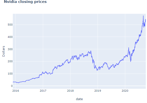
First, we must check for its stationarity. In this case our graph clearly shows that it is not stationary but in some cases it may look stationary but not actually so, therefore it is always good practice to check using one of three tests I've mentioned above.
In this blog I will use Augmented Dickey Fuller Test. We will use adfuller from statsmodel library. To test stationarity we use hypothesis testing where our null hypothesis would be "time series data is non-stationary". We will reject null hypothesis when p-value is less than 0.05(p-value) which makes us take alternative hypothesis "time series data is stationary".
from statsmodels.tsa.stattools import adfuller, acf, pacf

dftest = adfuller(nvda_df["Close"], autolag="AIC") #autolag = Method to use when automatically determining the lag

dfoutput = pd.Series(dftest[0:4], index=["Test Stats", "p-value", "# Lags", "# of obs"])
for key, value in dftest[4].items():
    dfoutput[f"Critical Value ({key})"] = value
print(dfoutput)

>>> Test Stats                 1.812313
>>> p-value                    0.998373
>>> # Lags                    13.000000
>>> # of obs                1189.000000
>>> Critical Value (1%)       -3.435862
>>> Critical Value (5%)       -2.863974
>>> Critical Value (10%)      -2.568066
p-value is very high therefore we cannot reject null hypothesis thus conclude that time series data is non-stationary. Don't give up yet, we can make it stationary by differencing our dependent variable.
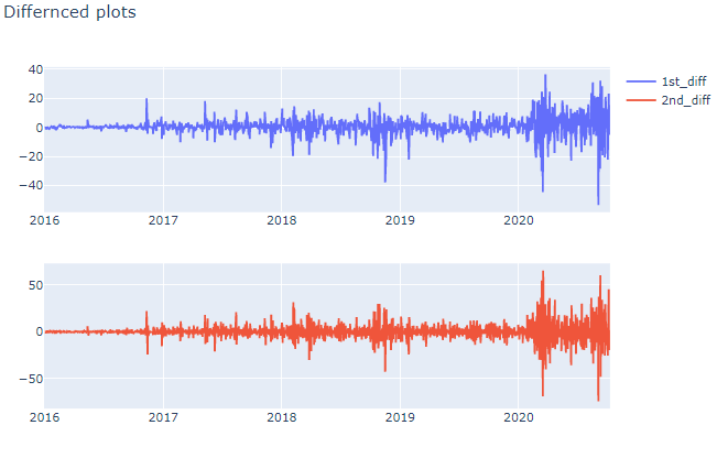
nvda_df["1st_diff"] = nvda_df["Close"].diff()
nvda_df["2nd_diff"] = nvda_df["1st_diff"].diff()

fig = make_subplots(rows=2, cols=1)

for idx, d in enumerate(["1st_diff", "2nd_diff"]):
    fig.add_trace(
        go.Scatter(
            name = d,
            x = nvda_df.index,
            y = nvda_df[d]
        ),
        row=idx+1,col=1
    )
fig.update_layout(
    title="Differnced plots"
)
fig.show()

plot_acf(nvda_df["1st_diff"].dropna());
Even with 1st order differencing our data became stationary.
Below is autocorrelation plot of 1st order differncing. You can see that even with one lag it lead to negative autocorrelation right away which indicates over-differncing. When autocorrelation decrease too fast it may indicate over-difference and if autocorrelation decrease too slow(stays positive for more than 10 lags) it indicates underdifferencing.
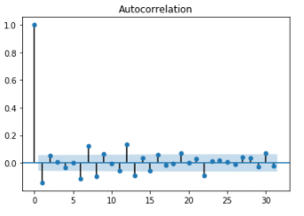
Also when time series is slightly under differenced, differencing once more lead to slight over differencing and vice versa. In such case instead of differencing add AR terms when slightly under-differenced and add MA terms when slightly over-differenced.
Forecasting
Finally time to use ARIMA model to make prediction. There is manual way to select q,d,p however since blog is getting too long I will explain it more deeper in later blogs and will show you easy way to select parameters.
import pmdarima as pm

model = pm.auto_arima(nvda_df.Close, start_p=1, start_q=1,
                      test='adf',       # use adftest to find optimal 'd'
                      max_p=3, max_q=3, # maximum p and q
                      m=1,              # frequency of series
                      d=None,           # let model determine 'd'
                      seasonal=False,   # No Seasonality
                      start_P=0,
                      D=0,
                      trace=True,
                      error_action='ignore',
                      suppress_warnings=True,
                      stepwise=True)
print(model.summary())
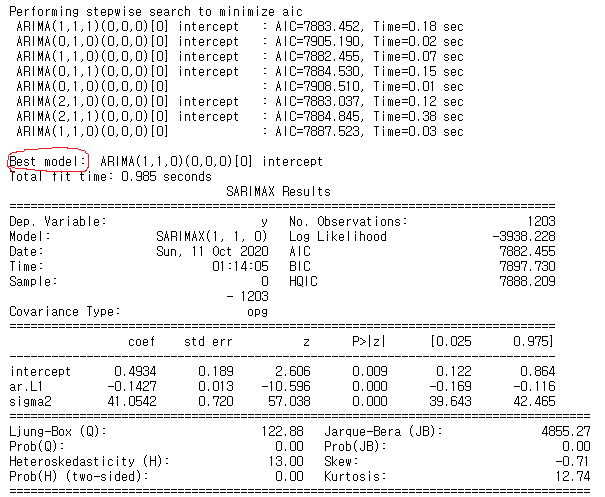
Above code tries all combination of p,d,q and output best model which is model with lowest AIC. Now create best ARIMA model and make predictions. Note that since it is time series data order matters therefore must split train and test data sequentially.
train = nvda_df.Close[:1000]
test  = nvda_df.Close[1000:]

model = ARIMA(train, order=(1, 1, 0))
fit_model = model.fit(disp=-1)

fc, se, conf = fit_model.forecast(203, alpha=0.05)  # 95% conf

fc_series    = pd.Series(fc, index=test.index)
lower_series = pd.Series(conf[:, 0], index=test.index)
upper_series = pd.Series(conf[:, 1], index=test.index)

plt.figure(figsize=(12,5), dpi=100)
plt.plot(train, label='training')
plt.plot(test, label='actual')
plt.plot(fc_series, label='forecast')
plt.fill_between(lower_series.index, lower_series, upper_series,
                    color='k', alpha=.15)
plt.title('Forecast vs Actuals')
plt.legend(loc='upper left', fontsize=8)
plt.show()
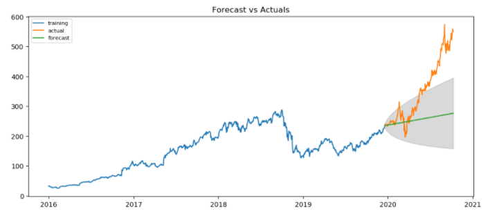
Precition doesn't seem to good. This is because ARIMA model does not account for irregularity and since Nvidia price sky rocketed due to events like CES and rise of self-driving vehicles our ARIMA model did a poor job.
Upto October 2018 there seems to be no irregularities. Lets truncate our data and see if it does well when there are no irregularities.
trunc_nvda_df = nvda_df[:"2018-10-01"].copy()
train = trunc_nvda_df.Close[:600]
test  = trunc_nvda_df.Close[600:]

model = ARIMA(train, order=(1, 1, 0))
fit_model = model.fit(disp=-1)

fc, se, conf = fit_model.forecast(93, alpha=0.05)  # 95% conf

fc_series    = pd.Series(fc, index=test.index)
lower_series = pd.Series(conf[:, 0], index=test.index)
upper_series = pd.Series(conf[:, 1], index=test.index)

plt.figure(figsize=(12,5), dpi=100)
plt.plot(train, label='training')
plt.plot(test, label='actual')
plt.plot(fc_series, label='forecast')
plt.fill_between(lower_series.index, lower_series, upper_series,
                    color='k', alpha=.15)
plt.title('Forecast vs Actuals')
plt.legend(loc='upper left', fontsize=8)
plt.show()
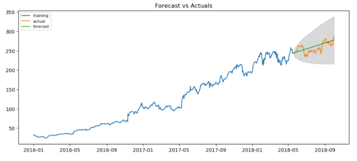
It does a very good job of predicting future stock prices Hooray!
In conclusion, ARIMA is works well in simple situations where there are no irregularities and no seasonality. In case of irregularities and seaonality you can use SARIMAX model which stands for Seasonal ARIMA model with eXogenous variables. ARIMA is a great base model if it does a great job, you use it and if it doesn't use more complex model but I always like to keep my model simple so I fully understand what is happening!
Thanks for reading my blog, have a great day!