Central Limit Theorem

date posted: 2020-07-12

Data distribution Vs. Sampling distribution

Before explaining Central limit theorem it is important to clearly understand difference between data and sampling distribution. Even though it is a very simple concept lot of people(including myself) get mixed up with the two leading to wrong assumption of central limit theorem.

Data Distribution: A function or listing showing all possible values of data, how often each data is likely to occur.
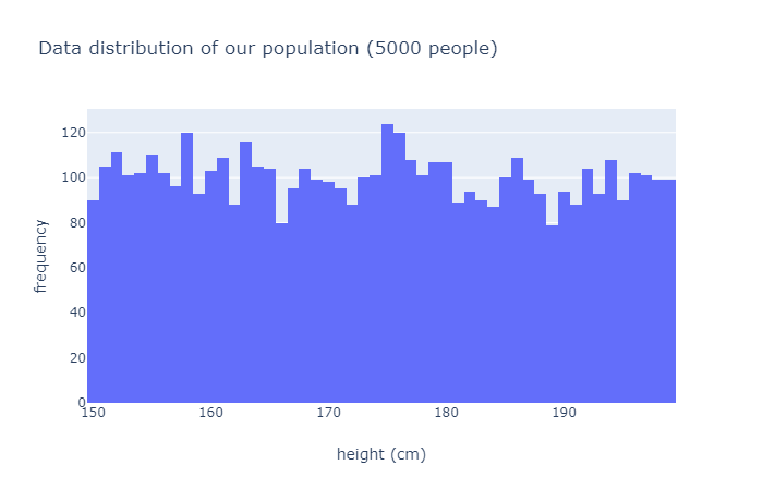
For example if we were to measure height of 5000 people each person's height would represent one data point and data distribution shows how many people are 160cm, 161cm and so on... Histogram is often used to represent data distribution.

import numpy as np
population =  np.random.randint(low=150, high=200, size=5000)

I will randomly choose 5000 people between 150 ~ 200cm height and create a data distribution (seen below).
It is a histogram representing frequency of data for each value of height. Left most bar indicate that there are about 90 people who are 150cm tall.

Sampling distribution: A function or listing showing all possible values of sample statistics from each sample, how often each sample statistic is likely to occur. From a population if we choose n samples and calculate sample statistic of our choice (mean, mode, median, etc...) that is one sample statistic, do this R times and distribute them on a histogram showing how likely each value of sample statistic is likely to occur, that is sampling distribution.

Central Limit Theorem

Definition: The tendency of sampling distribution to show shape of normal distribution as sampling size increases, often assumption that sampling distribution follows normal distribution is made when sampling size is greater than 30.

The key point here is that Central limit theorem is applied only to sampling distribution and not data distribution. Furthermore sampling size mentioned is talking about number of sampling statistic calculated.

Example

Now I will show you central limit theorem holding true in sampling distribution but not in data distribution.

Let's say we measured height of n number of people and create a histogram(data distribution) to see if it becomes similar to normal distribution as n increases.

fig = make_subplots(rows=5, cols=1,
subplot_titles=("n = 10", "n = 30", "n = 50", "n = 100", "n = 200"))

for idx, n in enumerate([10,30,50,100,200]):
    samples = np.random.randint(low=150, high=200, size=n)
    fig.add_trace(
        go.Histogram(
        x     = samples,
        name  = f"height of {n} people",
        xbins = dict(size=1)
        ),
        row=idx+1, col=1
    )
fig.update_layout(title = "Data distribution of height of n people",
height=800, width=800)
fig.show()

Below shows data distribution of sample size = 10, 30, 50, 100, 200 and it is clear to us that increasing n does not make data distribution close to normal distribution.

Now from our population of 5000 people I will measure height of 100 people and calculate their mean height (sample statistic). I will repeat it n times and show that as n increases sampling distribution will become more and more like bell-curve shaped(normal distribution). Note that mean height of 100 people is one sample size.

import random
fig = make_subplots(rows=6, cols=1,
                subplot_titles=("n = 10", "n = 30", "n = 50", "n = 100", "n = 200", "n=1000"))

for idx, n in enumerate([10,30,50,100, 200, 1000]):
    sampling_dist = []
    for i in range(n):
        samples       = random.sample(list(population), 100)
        sample_stats  = np.mean(samples) # note that it can be any statistics not just MEAN
        sampling_dist.append(sample_stats)

    fig.add_trace(
        go.Histogram(
            x     = sampling_dist,
            name  = f"mean height of {n} samples"
        ),
        row=idx+1, col=1
    )
fig.update_layout(title = "Sampling distribution of mean height of n people",
                    height=800, width=800)
fig.show()

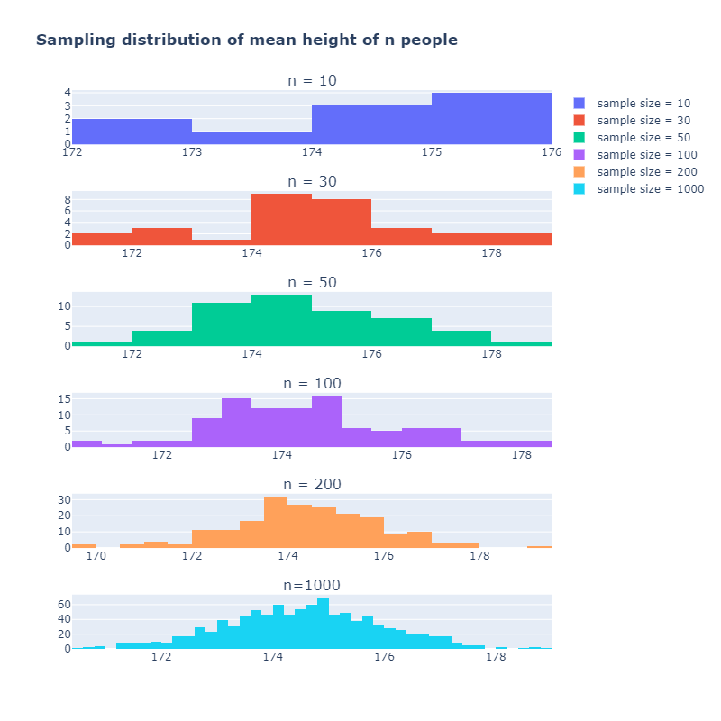
Note that sampling distribution becomes more like normal distribution as sample size increases. I've just showed you that central limit theorem only applies to sampling distribution so do not make a common mistake of assuming data distribution follows normal distribution when there are lots of data points.

One more thing, no matter what shape of population's data distribution follows when you create sampling distribution with large enough sample size central limit theorem will always hold true. No matter whether data distribution of population is skewed, bi-modal, etc... assumption of normal distribution is plausible when sample size is large enough.

Why assumption of normal distribution important?

Normal distribution leads to simpler mathematical calculations for distributions such as binomial and poisson. Even though binomial and poisson distribution can be calculated using their own function when assumption of normal distribution is made it makes the calculation much easier. Furthermore lots of data collected from real life are normally distributed such as height, reading ability, and more. Lastly once distribution is normal you could use empirical rule to see how far your data is deviated from the mean with ease.